
11 Regresión
There are two types of basic numerical techniques: interpolation and approximation (adjustment).
- The goal is to get a function that fits the best of your ability to a set of data (a cloud of data) from observations, data collected from sensors, datasets, etc.
- The simplest fitting model is the linear model (LM) named in Machine Learning community as linear regression.
- Although regression is probably the most simple approach for supervised learning, linear regression is still a useful and widely used statistical learning method.
- Other more complex statistical learning approaches are generalizations of linear regression.
11.1 Linear interpolation
The normal input is a data table \[\{(x_i,y_i)\}\]
And the goal is to find an interpolating function \[ \phi(x)=a_0+a_{1}f_{1}(x)\] (the easiest approach considers polynomial functions \(f_1(x)=x\)).
Then, the model will be:
\[ \phi(x)=a_0+a_{1}x\]
Existence and uniqueness of the solution
Simply, if we consider that \(\phi(x)\) verifies the conditions \((x_i,y_i)\), the following linear system is buit:
\[ \left. \begin{array}{ll}
a_0+a_{1}x_{1}&=y_{1}\\
a_0+a_{1}x_{2}&=y_{2}\\
\ldots&\ldots\\
a_0+a_{1}x_{m}&=y_{m}\\
\end{array}\right\}\]
Solving the system above, the coefficients \(a_0\) and \(a_{1}\) are obtained (if they exist) and we will have the Interpolation function: \[ \phi (x)=a_0+a_{1}x\]
- \(a_0\) is named the intercept.
- \(a_1\) is named the slope.
The condition for existence of the interpolation function \(\phi(x)\) is that the system should be consistent, its uniqueness depends on the solution(s) of the system.
11.2 Polynomial interpolation
Assuming we have \(n+1\) points \[\{ (x_{0}, y_{0}), (x_{1}, y_{1}), (x_{2}, y_{2}), \ldots, (x_{n}, y_{n})\} \] polynomial interpolation consists of finding a polynomial function \(\phi(x)\) passing through the given points.
\[ \phi (x)=a_0+a_{1}x+a_{2}x^2+\ldots+a_{n}x^n\] Note that we are using that a basis of the polynomials of grade less than or equal to \(n\) is \(B=\{1, x,x^2,\ldots,x^n\}\).
The equations will be:
\[ \left. \begin{array}{lr} a_0+a_{1}x_{0}+a_{2}x_{0}^2+\ldots&=y_{0}\\ a_0+a_{1}x_{1}+a_{2}x_{1}^2+\ldots&=y_{1}\\ \ldots&\ldots\\ a_0+a_{1}x_{n}+a_{2}x_{n}^2+\ldots&=y_{n}\\ \\ \end{array}\right\}\]
11.3 Linear Regression: Minimizing the residual sum of squares
With a large number of observations, interpolation methods are not adequate, hence an adjusting linear regression model \(y=\phi(x)\) is used. Such a model reflects the effect of changing a variable \(x\) (independent variable) in variable \(y\) (dependent variable). It considers that there exist a linear relationship between the variables.
A common way to estimate the parameters of a statistical model is to adjust a function which minimize the errors. The most used method is that of minimizing the residual sum of squares, RSS, which is defined by: \[ RSS(a)={\mid\mid \epsilon \mid\mid_2}^2= \displaystyle\sum_{i=1}^{N}{\epsilon_i}^2=\displaystyle\sum_{i=1}^{N}(y_i-a^TX)^2 \]
We compute the adjusting function which minimizes the RSS.
11.4 Linear Regression in R
The easier model is linear regression:
\[ \phi(x) = a_0 + a_1 x\]
Goal:
- Prediction of future observations.
- Find relationships, functions between dataset variables.
- Description of the data structure.
In mathematical terms, regression is to find a linear function that approaches the data cloud.
The lm() function is used to build a linear model:
regression.model <- lm( formula = y ~ x,
data = dataset ) - y is the dependent variable, the output.
- x is the independent variable, the predictor
- dataset a dataset with the attributes x and y
# execute only the fist time
# install.packages("readr")
require(readr)
library(readr)
CPIdata <- read_csv("data/EconomistData.csv")
#View(CPIdata)
attach(CPIdata)

# lm is a model formula
# ~ (read "is modeled as")
f1 <- lm(CPI ~ HDI)
f1
Call:
lm(formula = CPI ~ HDI)

Coefficients:
(Intercept)          HDI
-1.540 8.497 plot(HDI,CPI)
abline(f1) 
The linear model is \[\phi(x)=-1.540 + 8.497x\]
Which is the meaning of the coefficient \(8.497\)? - If \(x\) is increased in 1, then \(Y\) is increased in 1 Which is the meaning of the coefficient -1.540? - Value expected of \(y\), if \(x\) has the value 0
11.5 Evaluate the model
- Does the data fit the model found?
- Trying a more complicated model?: Polynomial regression.
- If the point cloud is \(n\) in size, interpolation can be achieved with a polynomial grade of \(n-1\).
- Very high grade polynomials introduce errors: oscillations, cost of computation, etc.
- For each model found, calculate in R the errors made, the accuracy, etc.
summary(f1)
Call:
lm(formula = CPI ~ HDI)

Residuals:
    Min      1Q  Median      3Q     Max
-2.9180 -1.1872 -0.2029  1.0744  3.4453

Coefficients:
            Estimate Std. Error t value Pr(>|t|)
(Intercept)  -1.5400     0.4453  -3.458 0.000686 ***
HDI           8.4975     0.6539  12.994  < 2e-16 ***
---
Signif. codes:  0 '***' 0.001 '**' 0.01 '*' 0.05 '.' 0.1 ' ' 1

Residual standard error: 1.506 on 171 degrees of freedom
Multiple R-squared:  0.4968,    Adjusted R-squared:  0.4939
F-statistic: 168.9 on 1 and 171 DF,  p-value: < 2.2e-16
#Explain the main estimatorsThere is some measures of the accuracy of the model.
We define the Residual Standard Error as follows: \[RSE=\sqrt{\frac{1}{n-2} \,\, RSS}\]
RSE is an estimate of the standard deviation of \(\epsilon_i\).
RSE is considered a measure of the lack of fit of the model to the data.
If the predictions using the model are very good, we can conclude that the model fits the data very well.
On the other hand, if the model doesn’t fit the data well then the RSE may be quite large.
R-squared (called the coefficient of determination) or fraction of variance explained is
\[R^2=1-\frac{RSS}{TSS}\] where \[TSS=\sum_{i=1}^n (y_i-\overline{y})\]
RSE is an absolute measure of lack of fit of the model.
\(R^2\) takes the form of a proportion measure (the proportion of variance explained), that is, the proportion of the variance in the outcome variable that can be accounted for by the predictor.
\(R^2\) can be estimated with the correlation \(r\) between the input (\(X\) variable) and the output (\(Y\) variable) as follows: \(R^2=r^2\).
If \(R^2\) is close to 1 indicates that a large proportion of the variability in the response has been explained by the regression. A number near 0 indicates that the linear model is wrong, or the inherent error is high, or both.
Note: The Pearson correlation is equivalent to running a linear regression model that uses only one predictor variable - the squared correlation \(r^2\) is identical to the \(R^2\) value for a linear regression with only a single predictor.
R language returns Multiple R-squared and Adjusted R-squared.
If you add more predictors into the model, the \(R^2\) value will increase (or at least it will be the same). In a regression model with \(K\) predictors, fit to a data set containing \(N\) observations, the adjusted \(R^2\) is:
\[ \mbox{adj. } R^2 = 1 - \left(\frac{\mbox{SS}_{res}}{\mbox{SS}_{tot}} \times \frac{N-1}{N-K-1} \right) \]
The adjusted \(R^2\) value will only increase when the new variables improve the model performance.
11.6 Model validation
- It is important to evaluate how the model adjusts the point cloud.
- There are many ways to make this assessment.
- Usually statisticians examine diagnostic plots after constructing the model.
- Most evaluation models focus on residuals
If we call \(\phi(x)\) to the regression linear function, at each point the error (residual) function is \[e (x_i)=\mid \phi(x_i)-y_i\mid \]
We assume these errors:
- They must have a zero average.
- If this is not the case, the bias must be measured.
- More points may need to be included in the data cloud.
- Errors must be uniformly distributed.
- We must wait for the residues to be uniformly distributed without patterns that detect anomalies.
- A first way would be to face the waste with the adjustment and the points should be around \(y=0\).
plot(fitted(f1), residuals(f1), xlab = "Approached values",  ylab = "Residuals")
abline(h=0, lty=2)
 lines(smooth.spline(fitted(f1), residuals(f1)))
 # See help of:
 #?fitted
 #?residuals
 #?smooth.spline
11.7 Generalized Regression
The linear model \(\phi(x) = a_0 + a_1 x\) could be generalized in several ways.
We can also apply linear regression to more than 1 variable \(x=\{x_1, x_2\}\).
For example, consider modeling temperature as a function of location \(\{x_1,x_2\}\).
\[ \phi(x) = a_0 + a_1 x_1 + a_2x_2\] or even, \[ \phi_2(x) =a_0 + a_1x_1 + a_2x_2 + a_3x_1^2\]
Note: it is possible to model non-linear relationships. In general, a simple approach (we could use non-polynomial functions) is considered using polynomial basis functions, where the model has the form
\[\phi(x)=a_0+a_1x+a_2x^2+ \ldots+ a_nx^n\]
Given a set of variables \(X_1, X_2, \dots, X_m\), multiple linear regression computes the next model:
\[\phi(x)=a_o+a_1X_1+a_2X_2+\dots, a_mX_m+\epsilon\] In this model a coefficient \(a_j\) is interpreted as the average effect on \(Y\) of a one unit increase in \(X_j\), holding all other predictors fixed.
The ideal scenario is when the predictors are uncorrelated and in this case each coefficient can be estimated and tested separately.
Correlations amongst predictors cause problems because the variance of all coefficients tends to increase, sometimes dramatically.
Normally the independence is a utopia. Normally, predictors usually change together.
# execute only the fist time
# install.packages("readr")
require(readr)
library(readr)
CPIdata <- read_csv("data/EconomistData.csv")
New names:
Rows: 173 Columns: 6
── Column specification
──────────────────────────────────────────────────────── Delimiter: "," chr
(2): Country, Region dbl (4): ...1, HDI.Rank, HDI, CPI
ℹ Use `spec()` to retrieve the full column specification for this data. ℹ
Specify the column types or set `show_col_types = FALSE` to quiet this message.
• `` -> `...1`#View(CPIdata)
attach(CPIdata)The following objects are masked from CPIdata (pos = 3):
...1, Country, CPI, HDI, HDI.Rank, Region
The following objects are masked from CPIdata (pos = 4):
...1, Country, CPI, HDI, HDI.Rank, Region# f(HDI.Rank)=a CPI + b HDI
modelo1 <- lm( HDI.Rank ~ CPI + HDI )
modelo1
Call:
lm(formula = HDI.Rank ~ CPI + HDI)

Coefficients:
(Intercept)          CPI          HDI
293.991 -2.935 -283.876 coef(modelo1)(Intercept) CPI HDI
293.991367 -2.935028 -283.876464 head(residuals(modelo1)) 1 2 3 4 5 6
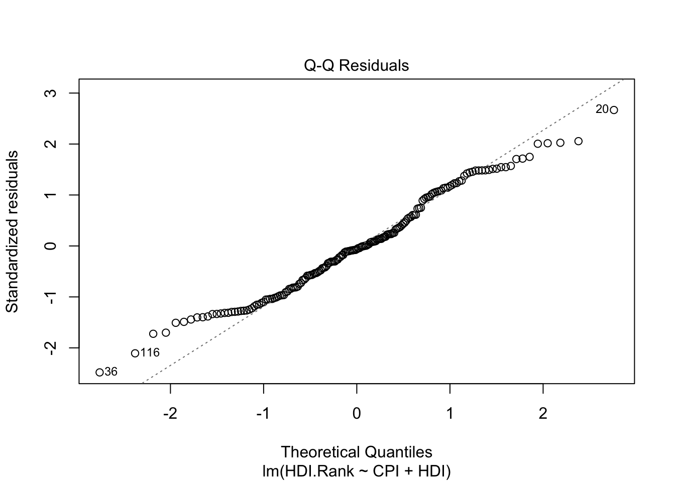
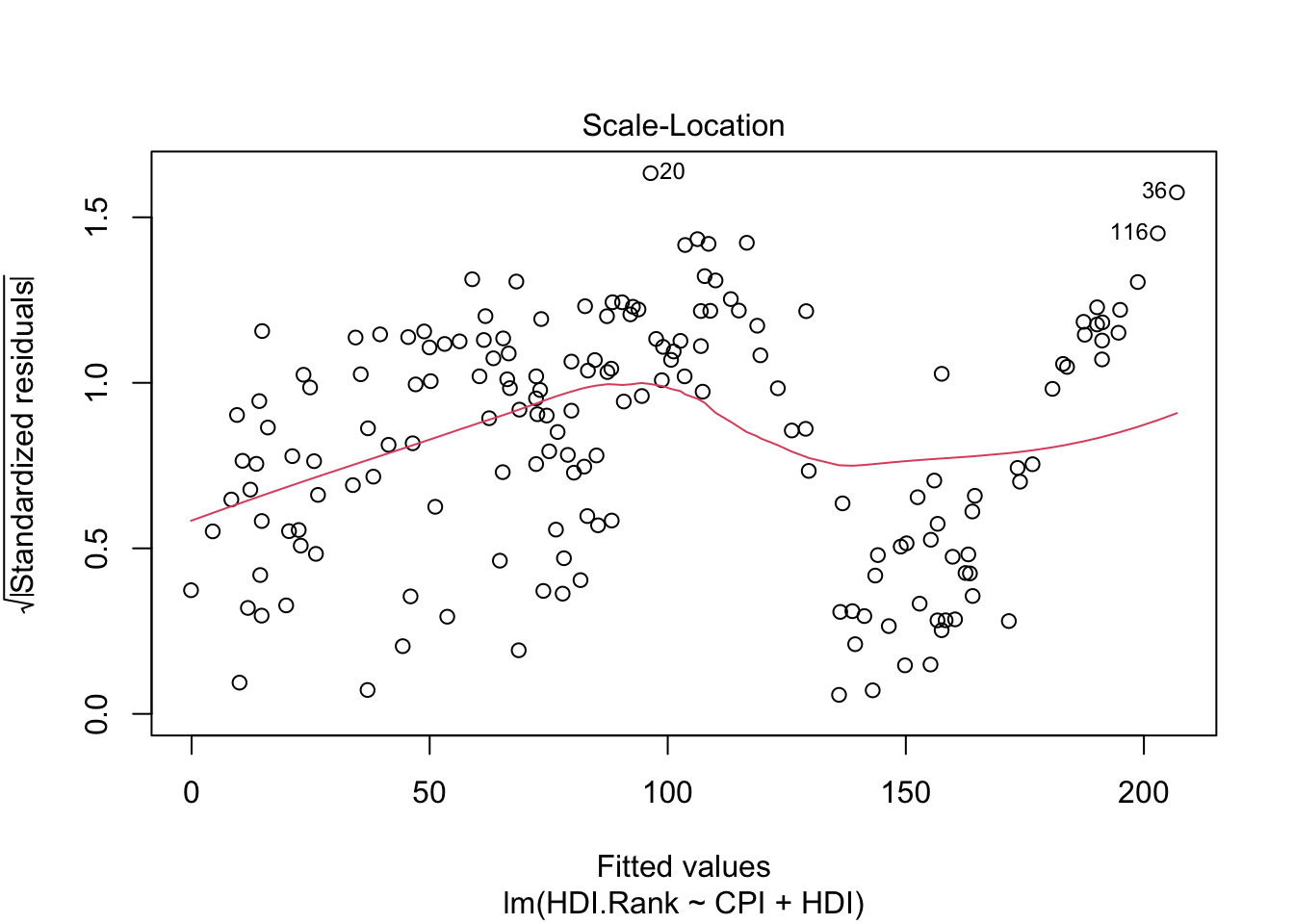
-4.605992 -5.108072 8.665987 -2.157349 -13.936740 2.895255 plot(modelo1)


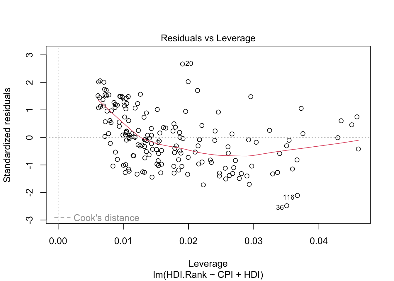
About plot(model):
The first plot (residuals vs. fitted values) is a simple scatterplot between residuals and predicted values. R shows some outliers.
The second plot (normal Q-Q) is a normal probability plot. It will give a straight line if the errors are distributed normally. Outliers deviate from the straight line.
The third plot (Scale-Location), like the the first, should look random. No patterns. We have a little V-shaped pattern.
The last plot (Cook’s distance) tells us which points have the greatest influence on the regression (leverage points). We see that points 20,36, 116 have great influence on the model. Detection of outliers: Remove these points and repeat.
11.8 Evaluating the Regression Coefficients
\[\phi(x)=a_o+a_1X_1+a_2X_2+\dots, a_pX_p\]
F-statistic:
We establish the null hypothesis.
\[H_O: a_o = a_1 = a_2= \dots= a_p= 0\]
versus the alternative \[H_a: \mbox{ at least one } a_i \mbox{ is non-zero}\]
The hyphotesis test is performed by means of F-statistic:
\[F=\frac{(TSS-RSS)/p}{RSS/(n-p-1)}\]
where
\[TSS = \sum (y_i − \overline{y} )^2\]
When there is no relationship between the real valor and predictors, the F-statistic must to take on a value close to 1.
If \(H_a\) is true the F-value must to be greater than 1.
If F-value is closer to 1, the answer to reject the hyphotesis depends on values of \(n\) and \(p\).
Using F-value, p-value is computed.
Using p-value we can determine whether or not to reject \(H_0\).
p-value is essentially 0: extremely strong evidence that at least one of the media is associated with output variable.
R language returns p-value for each coefficient: These provide information about whether each individual predictor is related to the response, after adjusting for the other predictors.
summary(modelo1)
Call:
lm(formula = HDI.Rank ~ CPI + HDI)

Residuals:
     Min       1Q   Median       3Q      Max
-19.9326  -6.5788  -0.5189   5.9769  21.6061

Coefficients:
             Estimate Std. Error t value Pr(>|t|)
(Intercept)  293.9914     2.5014 117.529  < 2e-16 ***
CPI           -2.9350     0.4153  -7.068 3.89e-11 ***
HDI         -283.8765     5.0064 -56.703  < 2e-16 ***
---
Signif. codes:  0 '***' 0.001 '**' 0.01 '*' 0.05 '.' 0.1 ' ' 1

Residual standard error: 8.178 on 170 degrees of freedom
Multiple R-squared:  0.9782,    Adjusted R-squared:  0.9779
F-statistic:  3806 on 2 and 170 DF,  p-value: < 2.2e-16
Pr(>|t|) of the coefficients is close to 0 (significatives) - see *** in each row of the table.
F-value is 3806 (must to be greater than 1).
p-value is close to 0.
degrees of freedom: The number of independent pieces of information used in the estimation of a parameter. From the algebaic point of view is the theal number of equations used from the data. (see Grados de libertad)
Multiple R-squared is used for evaluating how well your model fits the data. 97% of the variability in HDI.Rank is explained by CPI+HDI.
(Multiple R squared) measures the amount of variation in the response variable that can be explained by the predictor variables.
Adjusted Rsquared adds penalties for the number of predictors in the model. Therefore it shows a balance between the most parsimonious model, and the best fitting model ( ratio between the number of observations and the predictors). If you have a large difference between your multiple and your adjusted Rsquared that indicates you may have overfit your model.
11.9 Improving the models
Trying a more complicated model
- Polynomial regression.
- Polynomial ortogonal regression.
- Non linear regression.
- etc.
 p1 <- lm(CPI ~ HDI)
 p2 <- update(p1, . ~ . + I(HDI^2))
 p3 <- update(p2, . ~ . + I(HDI^3))
 p4 <- update(p3, . ~ . + I(HDI^4))
 p5 <- update(p4, . ~ . + I(HDI^5))
 p6 <- update(p5, . ~ . + I(HDI^6))
 p7 <- update(p6, . ~ . + I(HDI^7))
Using the previous example:
  require(readr)
  library(readr)
  CPIdata <- read_csv("data/EconomistData.csv")
New names:
Rows: 173 Columns: 6
── Column specification
──────────────────────────────────────────────────────── Delimiter: "," chr
(2): Country, Region dbl (4): ...1, HDI.Rank, HDI, CPI
ℹ Use `spec()` to retrieve the full column specification for this data. ℹ
Specify the column types or set `show_col_types = FALSE` to quiet this message.
• `` -> `...1`# View(CPIdata)
attach(CPIdata)The following objects are masked from CPIdata (pos = 3):
...1, Country, CPI, HDI, HDI.Rank, Region
The following objects are masked from CPIdata (pos = 4):
...1, Country, CPI, HDI, HDI.Rank, Region
The following objects are masked from CPIdata (pos = 5):
...1, Country, CPI, HDI, HDI.Rank, Region # lm is a model formula
# ~ (read "is modeled as")
f1 <- lm(CPI ~ HDI)
f1
Call:
lm(formula = CPI ~ HDI)

Coefficients:
(Intercept)          HDI
-1.540 8.497 plot(HDI,CPI)
abline(f1) 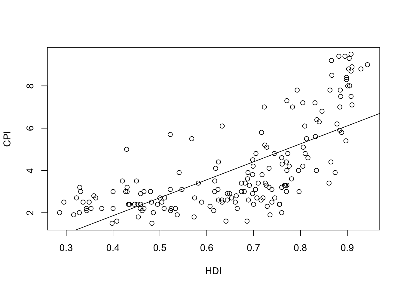
Computing errors: We develop a function that receives the model, the input variable, and computes the norm 2 of the vector of errors (eucliean distance):
\[\mid\mid \vec{e} \mid\mid= \sqrt{\sum (CPI_{i}-\phi(HDI_{i}))^2} \] - \(\phi(HDI_{i}))\) will be in the function y_aprox
require(pracma)#numerical packageLoading required package: pracmalibrary(pracma)
v.error <- function(Model,X,Y){
y_aprox <-predict(f1, data.frame(x = X))
r1 <- Y-y_aprox
nerror <- Norm(r1)
return(list(error.vector=r1, norma.error=nerror))
}#end function
# Compute errors with f1,HDI,CPI
mi.verror<-v.error(f1,HDI,CPI)
#norm 2 of the error
mie1 <- mi.verror$norma.error
mie1[1] 19.69212# Try
# mi.verror
# mi.verror$error.vector
# mi.verror$norma.errorIs this result coherent with residuals?
dif.myerror.resiuadls <- Norm(mi.verror$error.vector-residuals(f1))
dif.myerror.resiuadls
[1] 2.371631e-14We obtain the same values (taking in account rouning).
In any case the norm 2 of the errors in all the points of the dataset is 19.6921162 (computed using mi.verror$norma.error). In the following we will improve the model.
Before, we will examine the information computed in the building of the model (write f1$ and R will show all the possible parameters):
head(f1$model) CPI HDI
1 1.5 0.398
2 3.1 0.739
3 2.9 0.698
4 2.0 0.486
5 3.0 0.797
6 2.6 0.716head(f1$fitted.values) 1 2 3 4 5 6
1.841949 4.739580 4.391184 2.589725 5.232432 4.544139 # is the same that
# predict(f1, data.frame(x = HDI)
# the difference is:
Norm(f1$fitted.values-predict(f1, data.frame(x = HDI)))[1] 2.407623e-14Using orthogonal polynomials versus classical polynomial approach:
When we approach a function using classical approach - we minimize the norm 2 of the errors.
For this proposal we use in R language ``I(x^k)`` to add a term with k degree.
In R language we will use ``poly(x,k)`` to use orthogonal polynomials of k degree.
Trying a polynomial grade of \(n\) for \(\phi(x)\).
# Ajuste usando polinomios ortogonales

# Classical polynomial approach
# Usando I() para especificar que es una expresión matemática
poli.2c <- lm(CPI ~ HDI + I(HDI^2))
poli.3c <- lm(CPI ~ HDI + I(HDI^2) + I(HDI^3))
poli.4c <- lm(CPI ~ HDI + I(HDI^2) + I(HDI^3)+ I(HDI^4))
poli.2c
Call:
lm(formula = CPI ~ HDI + I(HDI^2))

Coefficients:
(Intercept)          HDI     I(HDI^2)
9.552 -30.051 30.785 poli.3c
Call:
lm(formula = CPI ~ HDI + I(HDI^2) + I(HDI^3))

Coefficients:
(Intercept)          HDI     I(HDI^2)     I(HDI^3)
-7.116 59.605 -119.817 80.060 poli.4c
Call:
lm(formula = CPI ~ HDI + I(HDI^2) + I(HDI^3) + I(HDI^4))

Coefficients:
(Intercept)          HDI     I(HDI^2)     I(HDI^3)     I(HDI^4)
   -0.08463      7.38593     18.62201    -75.89626     63.32330
# Orthogonal polynomial approach
# Usando poly() para especificar el grado de los polinomios ortogonales
poli.2o <- lm(CPI ~ poly(HDI, 2))
poli.3o <- lm(CPI ~ poly(HDI,3))
poli.4o <- lm(CPI ~ poly(HDI,4))
poli.2o
Call:
lm(formula = CPI ~ poly(HDI, 2))

Coefficients:
  (Intercept)  poly(HDI, 2)1  poly(HDI, 2)2
4.052 19.568 11.859 poli.3o
Call:
lm(formula = CPI ~ poly(HDI, 3))

Coefficients:
  (Intercept)  poly(HDI, 3)1  poly(HDI, 3)2  poly(HDI, 3)3
4.052 19.568 11.859 5.159 poli.4o
Call:
lm(formula = CPI ~ poly(HDI, 4))

Coefficients:
  (Intercept)  poly(HDI, 4)1  poly(HDI, 4)2  poly(HDI, 4)3  poly(HDI, 4)4
       4.0520        19.5681        11.8590         5.1587         0.6239
For each model found, calculate in R the errors made, the accuracy, etc.
The parameter $ Pr (>F)$ is the probability that rejecting null hypothesis (the most complex model does not fit better than the simplest model) could be an error.
Study of residuals:
Facing residues with the adjustment and points should be around y = 0.
plot(fitted(f1), residuals(f1), xlab = "Approached values",  ylab = "Residuals")
abline(h=0, lty=2)
 lines(smooth.spline(fitted(f1), residuals(f1)))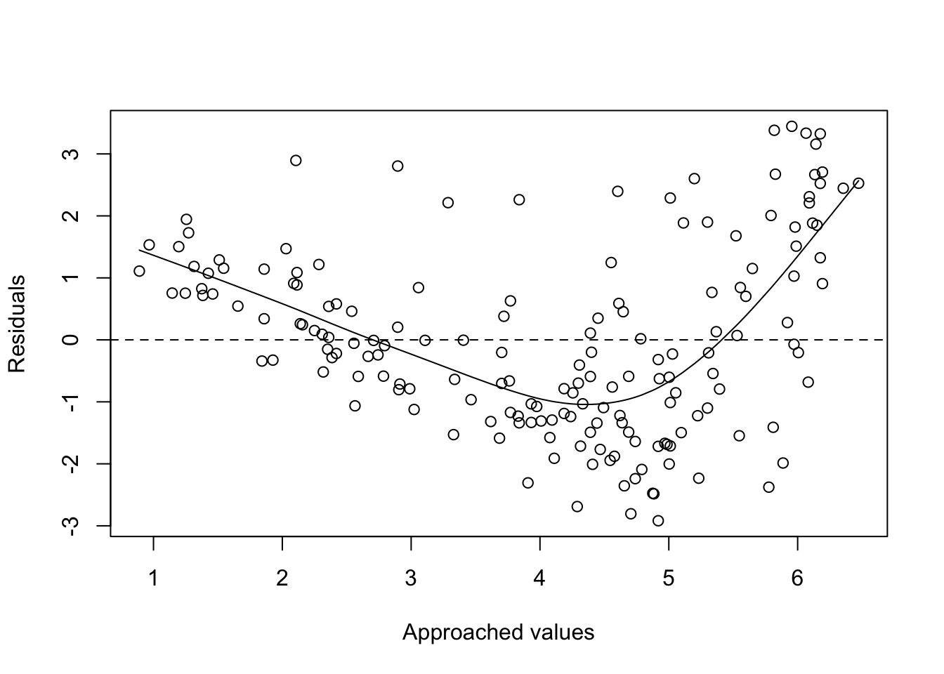
plot(fitted(poli.2o), residuals(poli.2o), xlab = "Approached values", ylab = "Residuals")

abline(h=0, lty=2)
lines(smooth.spline(fitted(poli.2o), residuals(poli.2o)))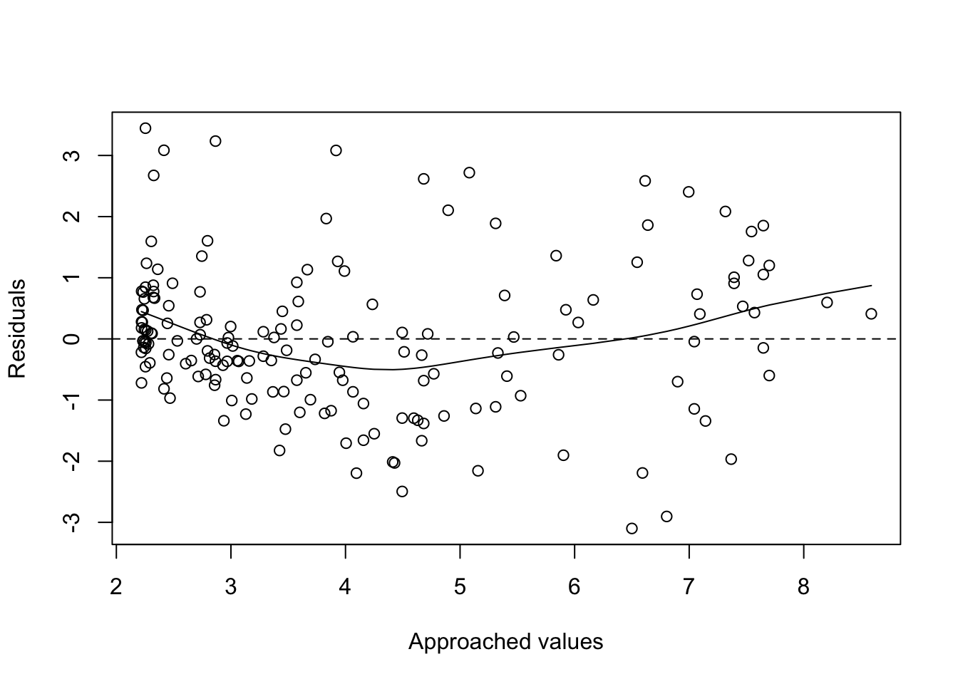
Another possibility would be to confront the residues with respect to the X-axis values. Points should be around \(y=0\).
Draw the point cloud next to the adjustment. Useful commands: predict, fitted. Estimators with residuals or draw the residuals
# 1
 plot(HDI, residuals(poli.2o), xlab = "HDI", ylab = "Residuos")
 abline(0, 0)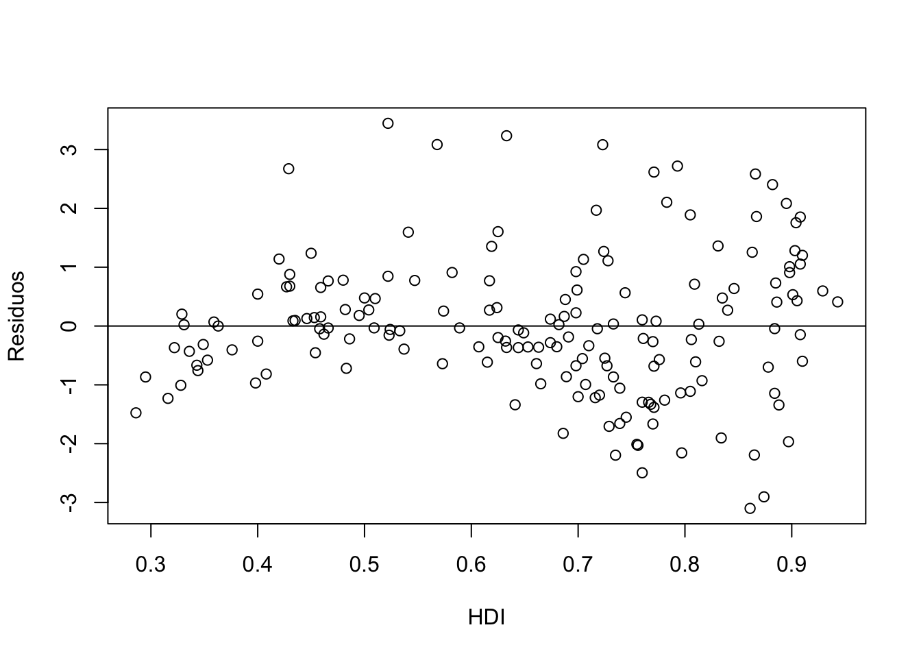
 # 2
 head(fitted(poli.2o))
1 2 3 4 5 6
2.468377 4.156869 3.575200 2.218723 5.156484 3.817822 head(predict(poli.2o, data.frame(x = HDI))) 1 2 3 4 5 6
2.468377 4.156869 3.575200 2.218723 5.156484 3.817822 plot(HDI,CPI,col="red")
par(new=TRUE)
plot(HDI,predict(poli.2o, data.frame(x = HDI)))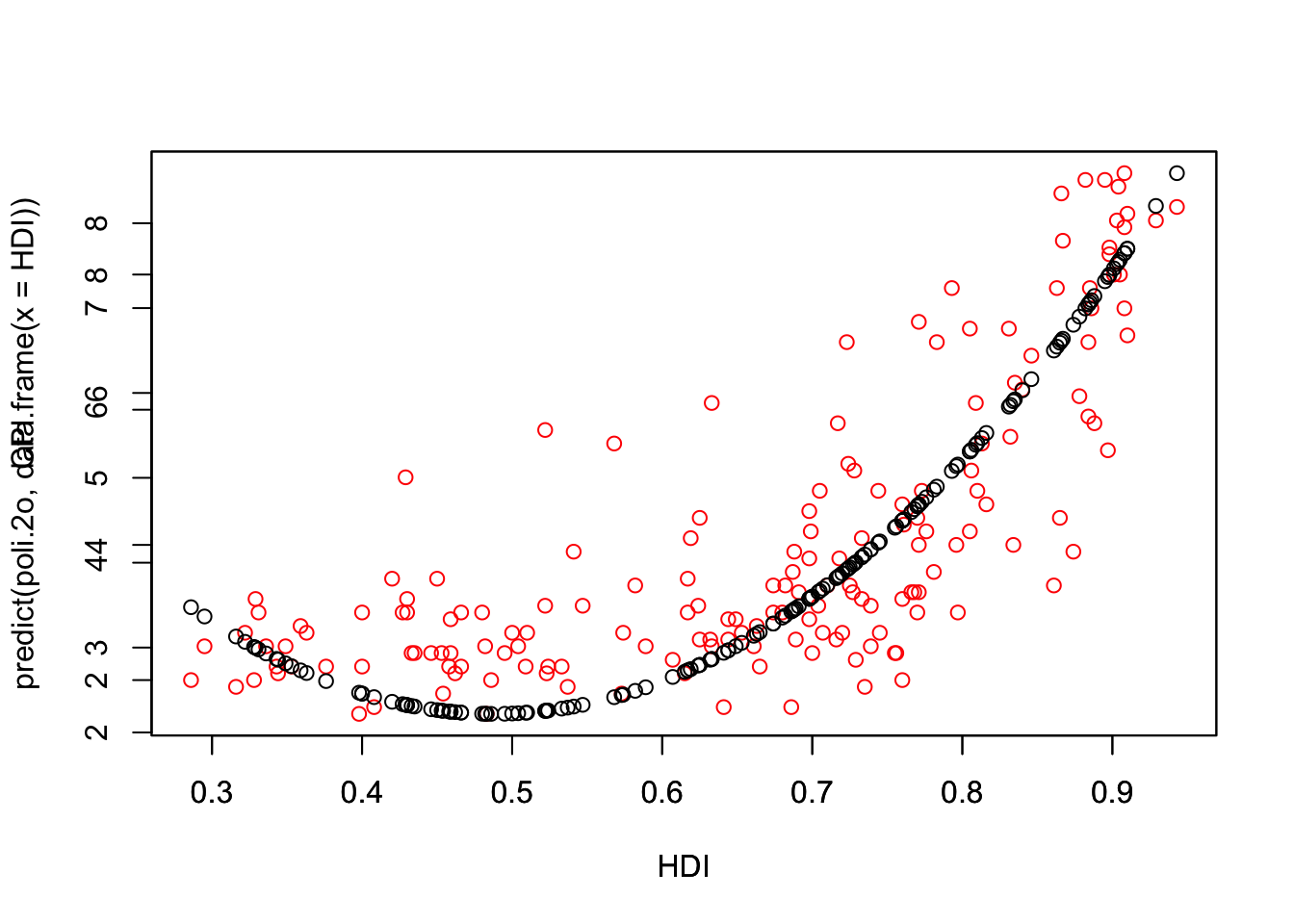
# predicted.intervals <- predict(poli.2o,data.frame(x=HDI),interval='confidence',
#                               level=0.99)
# lines(HDI,predicted.intervals[,1],col='firebrick1',lwd=3)

 # 3
 head(resid(poli.2o)) #List of residuals
1 2 3 4 5 6
-0.9683773 -1.0568692 -0.6752004 -0.2187232 -2.1564845 -1.2178223 mean(residuals(poli.2o)) [1] -2.053592e-17 plot(hist(resid(f1))) #A density plot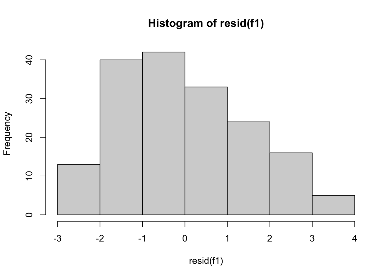
plot(density(resid(f1))) #A density plot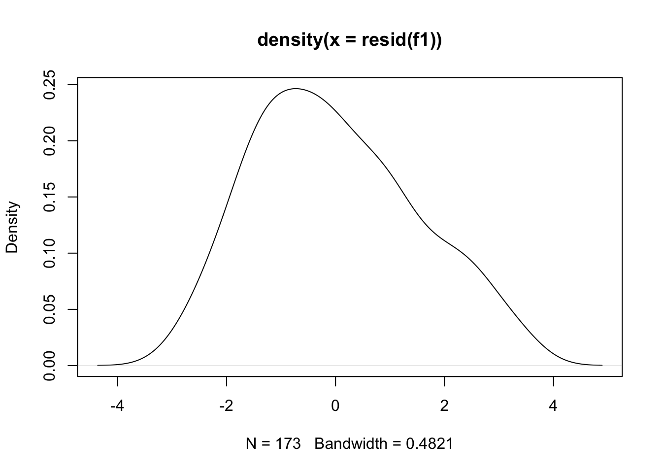
plot(density(resid(poli.2o))) #A density plot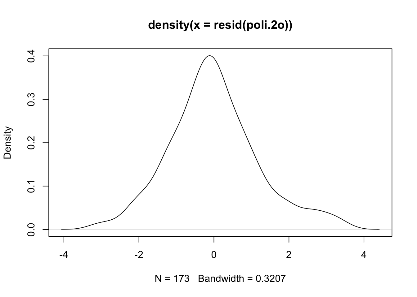
qqnorm(resid(poli.2o))

 qqline(resid(poli.2o))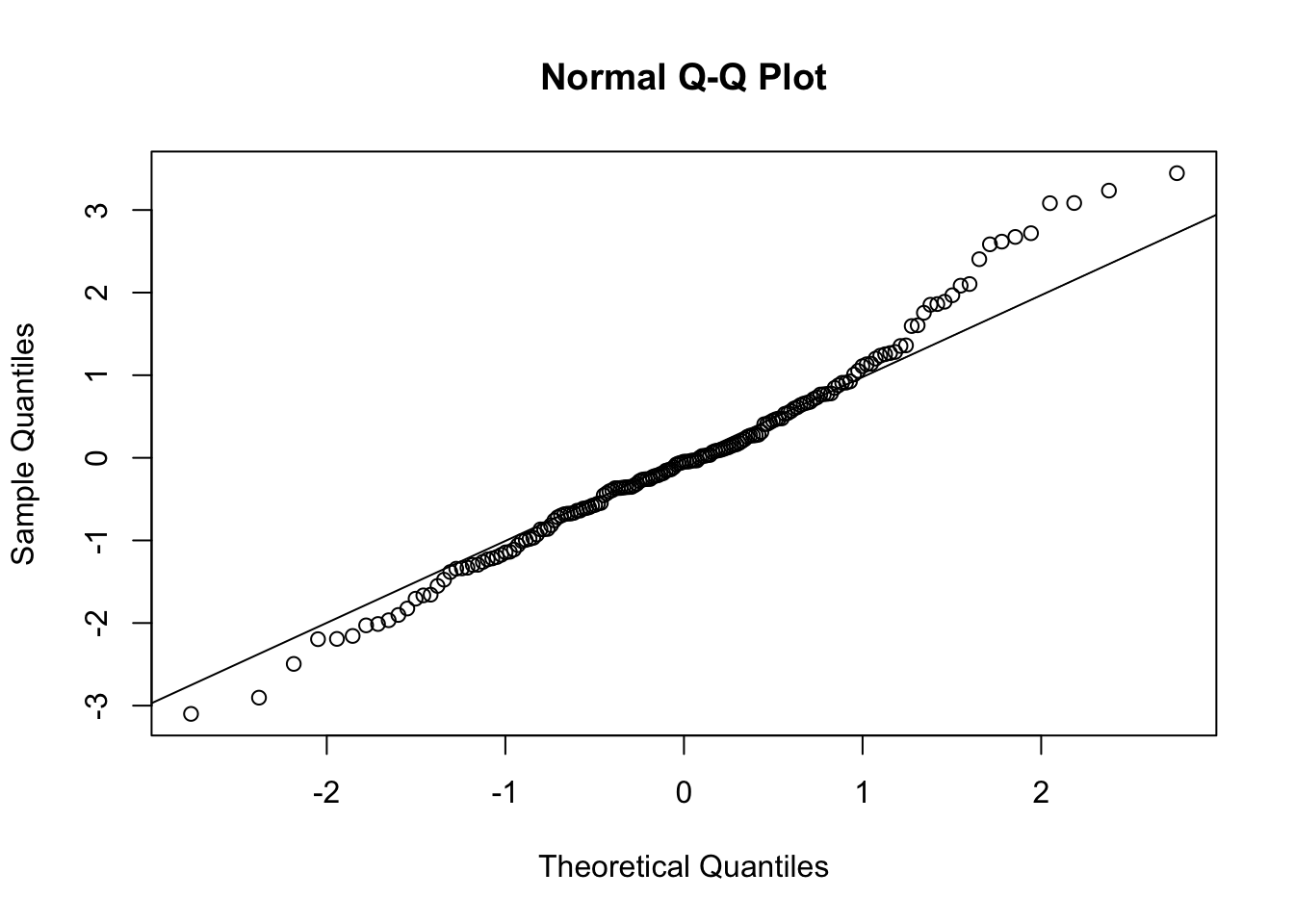
 #The deviations from the straight line are minimal. This indicates normal distribution.


# Quantile-quantile (QQ) plot.
# Evaluating the fit of sample data to the normal distribution.
# a plot of the sorted quantiles of one data set against the sorted quantiles of another data set.  It is used to visually inspect the similarity between the underlying distributions of 2 data sets.

 #Each point (x, y) is a plot of a quantile of one distribution along the vertical axis (y-axis) against the corresponding quantile of the other distribution along the horizontal axis (x-axis).
11.10 Searching the best regression
Given a set of variables \(A, B, X, Y, Z, U\) we can test the following models, in addition to the combinations of these with the linear and polynomial models previously seen.
- \(+\) para combinaciones de variables \(A+B\)
- \(.\) combinación de una de las variables con todas las demás
Examples:
# f1(X)=aY + bZ
f1 <- lm( X ~ Y + Z )

# f2(X)=a(Y+Z) + bU
f2 <- lm( X ~ I(Y + Z) + U )

#f3(X)=aY + bY^2+cZ
f3 <- lm( X ~ I(Y) + I(Y^2) + I(Z) )
f3 <- lm( X ~   Y + I(Y^2) +     Z )


# f5(X) interacciones entre X y todas las demás variables
f5 <- lm( X ~ . )
11.11 Dataset EconomistData
# execute only the fist time
# install.packages("readr")
require(readr)
library(readr)
CPIdata <- read_csv("data/EconomistData.csv")
New names:
Rows: 173 Columns: 6
── Column specification
──────────────────────────────────────────────────────── Delimiter: "," chr
(2): Country, Region dbl (4): ...1, HDI.Rank, HDI, CPI
ℹ Use `spec()` to retrieve the full column specification for this data. ℹ
Specify the column types or set `show_col_types = FALSE` to quiet this message.
• `` -> `...1`#View(CPIdata)
attach(CPIdata)The following objects are masked from CPIdata (pos = 4):
...1, Country, CPI, HDI, HDI.Rank, Region
The following objects are masked from CPIdata (pos = 5):
...1, Country, CPI, HDI, HDI.Rank, Region
The following objects are masked from CPIdata (pos = 6):
...1, Country, CPI, HDI, HDI.Rank, Region
The following objects are masked from CPIdata (pos = 7):
...1, Country, CPI, HDI, HDI.Rank, Region# f(HDI.Rank)=a CPI + b HDI
modelo1 <- lm( HDI.Rank ~ CPI + HDI )
plot(modelo1)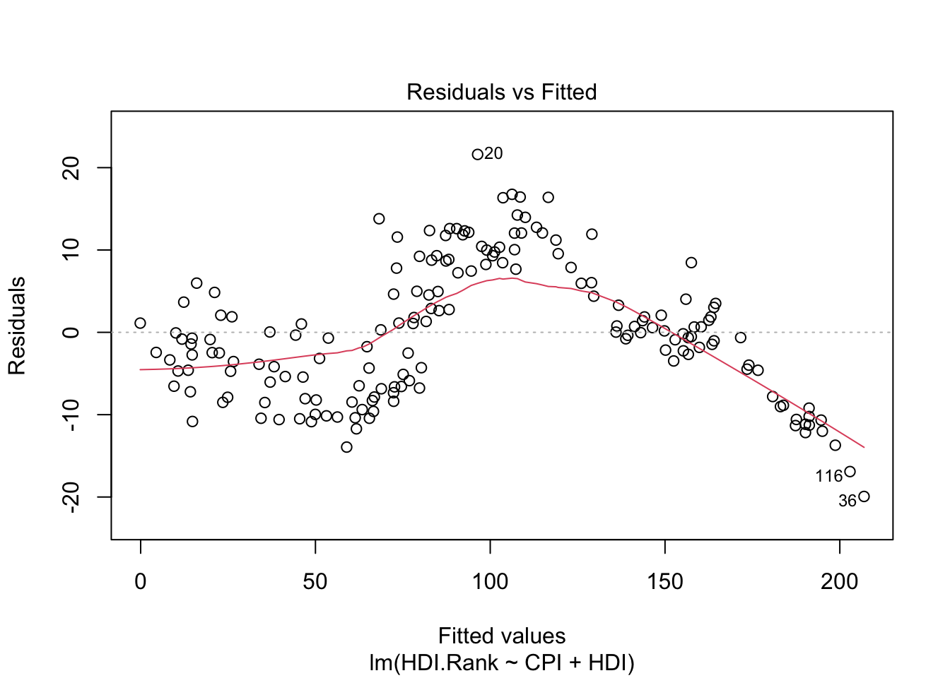

coef(modelo1)(Intercept) CPI HDI
293.991367 -2.935028 -283.876464 modelo1
Call:
lm(formula = HDI.Rank ~ CPI + HDI)

Coefficients:
(Intercept)          CPI          HDI
293.991 -2.935 -283.876 residuals(modelo1) 1 2 3 4 5 6
-4.60599167 -5.10807191 8.66598738 -2.15734861 -13.93673984 2.89525520
7 8 9 10 11 12
-2.44188161 -0.86747447 2.76622608 -0.69690560 -8.21829193 1.87144180
13 14 15 16 17 18
1.01589083 -7.33669193 -2.46410654 3.02896845 11.92180933 10.43680829
19 20 21 22 23 24
-2.51782785 21.60610822 4.98504226 1.88724332 -10.43701937 -10.22317210
25 26 27 28 29 30
-13.70985035 -0.36041659 0.17465976 -4.69679020 16.39312099 -11.16467728
31 32 33 34 35 36
-12.00982993 -0.33860867 12.59786618 4.54001917 -1.02878983 -19.93264142
37 38 39 40 41 42
0.77185089 0.30085876 -3.98371883 -10.28558786 -10.37611145 -6.04445802
43 44 45 46 47 48
-8.52410046 3.66733567 1.88059785 7.79734086 7.23059067 1.32426390
49 50 51 52 53 54
10.33665832 12.32046646 0.02684822 -10.58090997 -4.17033750 -9.01963378
55 56 57 58 59 60
5.97694164 -2.49937369 12.14645508 3.50934743 1.12369775 -4.60293950
61 62 63 64 65 66
6.03241096 -10.59463476 7.87830014 -12.17430366 -11.32591264 10.04000583
67 68 69 70 71 72
-1.82840115 12.06249696 -1.41606338 -10.84704151 -0.70956622 4.38764699
73 74 75 76 77 78
13.96549663 2.63386986 5.95289808 -7.21882433 -7.88590197 -10.43672650
79 80 81 82 83 84
1.07241621 -2.73844536 12.36203288 -6.57882450 -0.04118425 14.24613472
85 86 87 88 89 90
-8.50502517 -1.74412350 12.75621810 -0.78303728 -10.14369399 -5.86908897
91 92 93 94 95 96
4.02564135 -9.20391934 -8.37519745 -9.96329461 2.07726908 2.07442105
97 98 99 100 101 102
-0.63569608 -4.34075557 9.98854683 -8.86163679 -5.36998964 0.64873945
103 104 105 106 107 108
4.63934387 -9.60140437 9.75604064 9.30454080 -9.38249946 11.20383176
109 110 111 112 113 114
-10.65856881 -3.47649222 16.34554816 -0.51888391 -6.54203159 -3.34876745
115 116 117 118 119 120
9.54944141 -16.91023903 -0.64800176 1.11939457 9.22967666 1.41994197
121 122 123 124 125 126
-8.28864876 -2.24787220 8.24354415 1.79816613 8.45614978 -8.05714531
127 128 129 130 131 132
-5.43163410 0.04217940 -11.71774620 -6.62056839 8.46677827 13.79651559
133 134 135 136 137 138
11.57122268 11.76225118 -6.49236455 -0.18048754 -7.85640169 -8.46672378
139 140 141 142 143 144
-11.27130400 4.84791253 -10.49828222 -4.72790498 0.71020644 16.76178084
145 146 147 148 149 150
-3.55065523 8.85286350 -4.47372418 11.84971387 3.29073539 -0.07127899
151 152 153 154 155 156
-0.82266968 12.04963221 12.07221208 -0.89984945 12.59147817 0.57155095
157 158 159 160 161 162
-1.46103690 4.95625185 -6.85316332 9.30751297 8.76540081 7.44393283
163 164 165 166 167 168
0.66160421 -4.29485930 -3.87368502 -10.82508278 -3.17089656 7.66949195
169 170 171 172 173
16.43301085 -6.76561190 -2.67688090 1.46760353 -7.79675397 In the following, we check some models.
# INTERACCION ENTRE CPI y HDI
modelo1a = lm( HDI.Rank ~ ., data = CPIdata)

# modelo no lineal
modelo2a = lm( HDI.Rank ~ log(CPI) + HDI)

#  test others models
# modelo3a=
# modelo4a=.....