library(fcaR)10 FCA
History of FCA:
Port-Royal logic (traditional logic): formal notion of concept, Arnauld A., Nicole P.: La logique ou l’art de penser, 1662 (Logic Or The Art Of Thinking, CUP, 2003): concept = extent (objects) + intent (attributes)
G. Birkhoff (1940s): work on lattices and related mathematical structures, emphasizes applicational aspects of lattices in data analysis.
Barbut M., Monjardet B.: Ordre et classiffication, algebre et combinatoire. Hachette, Paris, 1970.
Wille R.: Restructuring lattice theory: an approach based on hierarchies of concepts. In: I. Rival (Ed.): Ordered Sets. Reidel, Dordrecht, 1982, pp. 445-470.
Ganter B., Wille R.: Formal Concept Analysis. Springer, 1999.
10.0.1 Application of FCA
- knowledge extraction
- clustering and classification
- machine learning
- concepts, ontologies
- rules, association rules, attribute implications
10.0.2 fcaR package
This is a summary of some of the functionalities introduced in package fcaR:
- Computing implications and concepts using Ganter’s algorithm.
- Visualization of the concept lattice.
- Removal of redundancies in implications.
- Computation of closures.
FCA provides methods to describe the relationship between a set of objects \(G\) and a set of attributes \(M\).
We show the main methods of FCA using the main functionalities and data structures of the fcaR package.
We load the fcaR package by:
Formal Context, \(\mathbf{K}:=(G,M,I)\)
objects <- c("Mercury", "Venus", "Earth", "Mars",
             "Jupiter", "Saturn", "Uranus", "Neptune",
             "Pluto")

attributes <- c("small", "medium", "large",
                "near", "far",
                "moon", "no_moon")

planets <- matrix(0, nrow = length(objects),
                  ncol = length(attributes))

rownames(planets) <- objects
colnames(planets) <- attributes

planets["Mercury", c("small", "near", "no_moon")] <- 1
planets["Venus", c("small", "near", "no_moon")] <- 1
planets["Earth", c("small", "near", "moon")] <- 1
planets["Mars", c("small", "near", "moon")] <- 1
planets["Jupiter", c("large", "far", "moon")] <- 1
planets["Saturn", c("large", "far", "moon")] <- 1
planets["Uranus", c("medium", "far", "moon")] <- 1
planets["Neptune", c("medium", "far", "moon")] <- 1
planets["Pluto", c("small", "far", "moon")] <- 1
fc_planets <- FormalContext$new(planets)knitr::kable(planets, format = "html", booktabs = TRUE)| small | medium | large | near | far | moon | no_moon | |
|---|---|---|---|---|---|---|---|
| Mercury | 1 | 0 | 0 | 1 | 0 | 0 | 1 |
| Venus | 1 | 0 | 0 | 1 | 0 | 0 | 1 |
| Earth | 1 | 0 | 0 | 1 | 0 | 1 | 0 |
| Mars | 1 | 0 | 0 | 1 | 0 | 1 | 0 |
| Jupiter | 0 | 0 | 1 | 0 | 1 | 1 | 0 |
| Saturn | 0 | 0 | 1 | 0 | 1 | 1 | 0 |
| Uranus | 0 | 1 | 0 | 0 | 1 | 1 | 0 |
| Neptune | 0 | 1 | 0 | 0 | 1 | 1 | 0 |
| Pluto | 1 | 0 | 0 | 0 | 1 | 1 | 0 |
Two mappings can be defined:
intent: \((\ )'\colon 2^G \to 2^M\) with, for all \(A\subseteq G\), \(A' = \{m \in M \mid g\, I\, m \mbox{ for all } g \in A\}\) for all \(A\subseteq G\).
extent: \((\ )'\colon 2^M \to 2^G\) with, for all \(B\subseteq M\), \(B' = \{g \in G \mid g\, I\, m \mbox{ for all } m \in B\}\).
That is, the intent of a set of objects is the set of their common attributes:
# Define a set of objects
S <- Set$new(attributes = fc_planets$objects)
S$assign(Earth = 1, Mars = 1)
cat("Given the set of objects:")
Given the set of objects:S{Earth, Mars}cat("The intent is:")The intent is:# Compute the intent of S
fc_planets$intent(S){small, near, moon}Analogously, the extent of a set of attributes is the set of objects which possess all the attributes in the given set:
# Define a set of objects
S <- Set$new(attributes = fc_planets$attributes)
S$assign(moon = 1, large = 1)
cat("Given the set of attributes:")
Given the set of attributes:S{large, moon}cat("The extent is:")The extent is:# Compute the extent of S
fc_planets$extent(S){Jupiter, Saturn}This pair of mappings is a Galois connection.
The composition of intent and extent is the closure of a set of attributes:
# Compute the closure of S
print("El conjunto de objetos ")
[1] "El conjunto de objetos "S{large, moon}print("tiene como cerrado")[1] "tiene como cerrado"Sc <- fc_planets$closure(S)
Sc{large, far, moon}This means that all planets which have the attributes moon and large also have far in common.
Definition: A formal concept is a pair \((A,B)\) such that \(A \subseteq G\), \(B \subseteq M\), \(A' = B\) and \(B' = A\). Consequently, \(A\) and \(B\) are closed sets of objects and attributes, respectively.
# Define a set of objects
S <- Set$new(attributes = fc_planets$attributes)
S$assign(moon = 1, large = 1, far= 1)
print("Given the set of attributes:")[1] "Given the set of attributes:"S{large, far, moon}print("The extent is:")[1] "The extent is:"# Compute the extent of S
extent <- fc_planets$extent(S)
extent{Jupiter, Saturn}print("And the intent of this one is:")[1] "And the intent of this one is:"fc_planets$intent(extent){large, far, moon}\(\big(\{Jupiter, Saturn\},\{large, far, moon\}\big)\) is a concept. It is a maximal cluster.
We are going to work with two datasets, a crisp one and a fuzzy one.
The classical (binary) dataset is the well-known planets formal context, presented in
Wille R (1982). “Restructuring Lattice Theory: An Approach Based on Hierarchies of Concepts.” In Ordered Sets, pp. 445–470. Springer.
objects <- c("Mercury", "Venus", "Earth", "Mars",
"Jupiter", "Saturn", "Uranus", "Neptune",
"Pluto")
attributes <- c("small", "medium", "large",
"near", "far",
"moon", "no_moon")
planets <- matrix(0, nrow = length(objects),
ncol = length(attributes))
rownames(planets) <- objects
colnames(planets) <- attributes
planets["Mercury", c("small", "near", "no_moon")] <- 1
planets["Venus", c("small", "near", "no_moon")] <- 1
planets["Earth", c("small", "near", "moon")] <- 1
planets["Mars", c("small", "near", "moon")] <- 1
planets["Jupiter", c("large", "far", "moon")] <- 1
planets["Saturn", c("large", "far", "moon")] <- 1
planets["Uranus", c("medium", "far", "moon")] <- 1
planets["Neptune", c("medium", "far", "moon")] <- 1
planets["Pluto", c("small", "far", "moon")] <- 1knitr::kable(planets, format = "html", booktabs = TRUE)| small | medium | large | near | far | moon | no_moon | |
|---|---|---|---|---|---|---|---|
| Mercury | 1 | 0 | 0 | 1 | 0 | 0 | 1 |
| Venus | 1 | 0 | 0 | 1 | 0 | 0 | 1 |
| Earth | 1 | 0 | 0 | 1 | 0 | 1 | 0 |
| Mars | 1 | 0 | 0 | 1 | 0 | 1 | 0 |
| Jupiter | 0 | 0 | 1 | 0 | 1 | 1 | 0 |
| Saturn | 0 | 0 | 1 | 0 | 1 | 1 | 0 |
| Uranus | 0 | 1 | 0 | 0 | 1 | 1 | 0 |
| Neptune | 0 | 1 | 0 | 0 | 1 | 1 | 0 |
| Pluto | 1 | 0 | 0 | 0 | 1 | 1 | 0 |
The other formal context is fuzzy and is defined by the following matrix I:
objects <- paste0("O", 1:6)
n_objects <- length(objects)
attributes <- paste0("P", 1:6)
n_attributes <- length(attributes)
I <- matrix(data = c(0, 1, 0.5, 0, 0, 0.5,
0, 1, 0.5, 0, 0, 0.5,
0.5, 1, 0, 0, 1, 0,
0.5, 0, 0, 1, 0.5, 0,
1, 0, 0, 0.5, 0, 0,
0, 0, 1, 0, 0, 1),
nrow = n_objects,
byrow = FALSE)
colnames(I) <- attributes
rownames(I) <- objects
fc_planets <- FormalContext$new(planets)
fc_I <- FormalContext$new(I)knitr::kable(I, format = "html", booktabs = TRUE)| P1 | P2 | P3 | P4 | P5 | P6 | |
|---|---|---|---|---|---|---|
| O1 | 0.0 | 0.0 | 0.5 | 0.5 | 1.0 | 0 |
| O2 | 1.0 | 1.0 | 1.0 | 0.0 | 0.0 | 0 |
| O3 | 0.5 | 0.5 | 0.0 | 0.0 | 0.0 | 1 |
| O4 | 0.0 | 0.0 | 0.0 | 1.0 | 0.5 | 0 |
| O5 | 0.0 | 0.0 | 1.0 | 0.5 | 0.0 | 0 |
| O6 | 0.5 | 0.5 | 0.0 | 0.0 | 0.0 | 1 |
10.0.3 Working with Formal Contexts
The first step when using the fcaR package to analyse a formal context is to create an object of class FormalContext which will store all the information related to the context.
In our examples, we create two objects:
fc_planets <- FormalContext$new(planets)
fc_I <- FormalContext$new(I)Internally, the object stores information about whether the context is binary or the names of objects and attributes, which are taken from the rownames and colnames of the provided matrix.
Once created the FormalContext objects, we can print them or plot them as heatmaps (with functions print() and plot()):
print(fc_planets)FormalContext with 9 objects and 7 attributes.
small medium large near far moon no_moon
Mercury X X X
Venus X X X
Earth X X X
Mars X X X
Jupiter X X X
Saturn X X X
Uranus X X X
Neptune X X X
Pluto X X X print(fc_I)FormalContext with 6 objects and 6 attributes.
P1 P2 P3 P4 P5 P6
O1 0 0 0.5 0.5 1 0
O2 1 1 1 0 0 0
O3 0.5 0.5 0 0 0 1
O4 0 0 0 1 0.5 0
O5 0 0 1 0.5 0 0
O6 0.5 0.5 0 0 0 1 fc_planets$plot()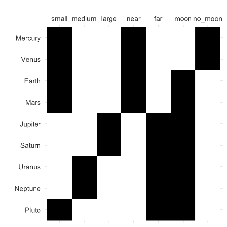
fc_I$plot()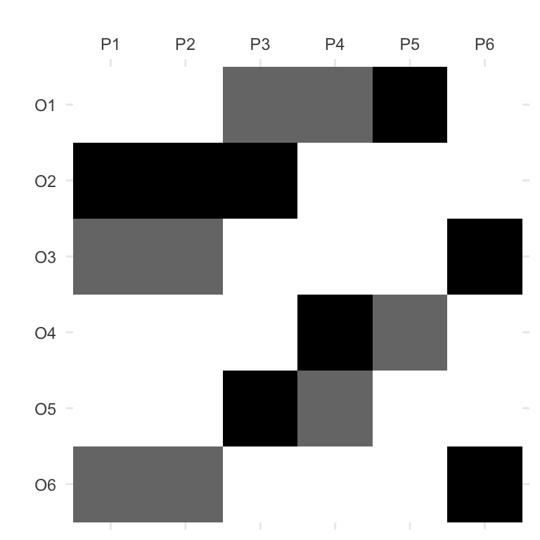
Also, we can export the formal context as a LaTeX table:
fc_planets$to_latex()\begin{table} \caption{}\label{} \centering \begin{tabular}{r|ccccccc}
& $small$ & $medium$ & $large$ & $near$ & $far$ & $moon$ & $no\_moon$\\
\hline
$Mercury$ & $\times$ & & & $\times$ & & & $\times$ \\
$Venus$ & $\times$ & & & $\times$ & & & $\times$ \\
$Earth$ & $\times$ & & & $\times$ & & $\times$ & \\
$Mars$ & $\times$ & & & $\times$ & & $\times$ & \\
$Jupiter$ & & & $\times$ & & $\times$ & $\times$ & \\
$Saturn$ & & & $\times$ & & $\times$ & $\times$ & \\
$Uranus$ & & $\times$ & & & $\times$ & $\times$ & \\
$Neptune$ & & $\times$ & & & $\times$ & $\times$ & \\
$Pluto$ & $\times$ & & & & $\times$ & $\times$ &
\end{tabular}
\end{table}The basic operation in FCA is the computation of closures given an attribute set, by using the two derivation operators, extent and intent.
The intent of a (probably fuzzy) set of objects is the set of their common attributes:
# Define a set of objects
S <- Set$new(attributes = fc_planets$objects)
S$assign(Earth = 1, Mars = 1)
S{Earth, Mars}# Compute the intent of S
fc_planets$intent(S){small, near, moon}Analogously, the extent of a set of attributes is the set of objects which possess all the attributes in the given set:
# Define a set of objects
S <- Set$new(attributes = fc_planets$attributes)
S$assign(moon = 1, large = 1)
S{large, moon}# Compute the extent of S
fc_planets$extent(S){Jupiter, Saturn}The composition of intent and extent is the closure of a set of attributes:
# Compute the closure of S
Sc <- fc_planets$closure(S)
Sc
{large, far, moon}This means that all planets which have the attributes moon and large also have far in common.
We can check whether a set is closed (that is, it is equal to its closure), using is_closed():
fc_planets$is_closed(S)[1] FALSEfc_planets$is_closed(Sc)[1] TRUEAn interesting point when managing formal contexts is the ability to reduce the context, removing redundancies, while retaining all the knowledge. This is accomplished by two functions: clarify(), which removes duplicated attributes and objects (columns and rows in the original matrix); and reduce(), which uses closures to remove dependent attributes, but only on binary formal contexts. The resulting FormalContext is equivalent to the original one in both cases.
fc_planets$reduce(TRUE)FormalContext with 5 objects and 7 attributes.
small medium large near far moon no_moon
Pluto X X X
[Mercury, Venus] X X X
[Earth, Mars] X X X
[Jupiter, Saturn] X X X
[Uranus, Neptune] X X X fc_I$clarify(TRUE)FormalContext with 5 objects and 5 attributes.
P3 P4 P5 P6 [P1, P2]
O1 0.5 0.5 1 0 0
O2 1 0 0 0 1
O4 0 1 0.5 0 0
O5 1 0.5 0 0 0
[O3, O6] 0 0 0 1 0.5 Note that merged attributes or objects are stored in the new formal context by using squared brackets to unify them, e.g. [Mercury, Venus].
The function to extract the canonical basis of implications and the concept lattice is find_implications(). Its use is to store a ConceptLattice and an ImplicationSet objects internally in the FormalContext object after running the NextClosure algorithm.
It can be used both for binary and fuzzy formal contexts, resulting in binary or fuzzy concepts and implications:
fc_planets$find_implications()

fc_I$find_implications()
We can inspect the results as:
# Concepts
fc_planets$concepts
A set of 12 concepts:
1: ({Mercury, Venus, Earth, Mars, Jupiter}, {})
2: ({Venus, Earth, Mars, Jupiter}, {moon})
3: ({Earth, Mars, Jupiter}, {far, moon})
4: ({Earth}, {large, far, moon})
5: ({Mars}, {medium, far, moon})
6: ({Mercury, Venus, Jupiter}, {small})
7: ({Venus, Jupiter}, {small, moon})
8: ({Jupiter}, {small, far, moon})
9: ({Mercury, Venus}, {small, near})
10: ({Mercury}, {small, near, no_moon})
11: ({Venus}, {small, near, moon})
12: ({}, {small, medium, large, near, far, moon, no_moon})# Implications
fc_planets$implicationsImplication set with 10 implications.
Rule 1: {no_moon} -> {small, near}
Rule 2: {far} -> {moon}
Rule 3: {near} -> {small}
Rule 4: {large} -> {far, moon}
Rule 5: {medium} -> {far, moon}
Rule 6: {medium, large, far, moon} -> {small, near, no_moon}
Rule 7: {small, near, moon, no_moon} -> {medium, large, far}
Rule 8: {small, near, far, moon} -> {medium, large, no_moon}
Rule 9: {small, large, far, moon} -> {medium, near, no_moon}
Rule 10: {small, medium, far, moon} -> {large, near, no_moon}A FormalContext is saved and loaded (in RDS format) using its own methods save() and load(), which are more efficient than the base saveRDS() and readRDS().
fc$save(filename = "./fc.rds")

# Create an empty FormalContext where to
# import the previously saved
fc2 <- FormalContext$new()
fc2$load("./fc.rds")
10.0.4 Concept Lattice
We are going to use the previously computed concept lattices for the two FormalContext objects.
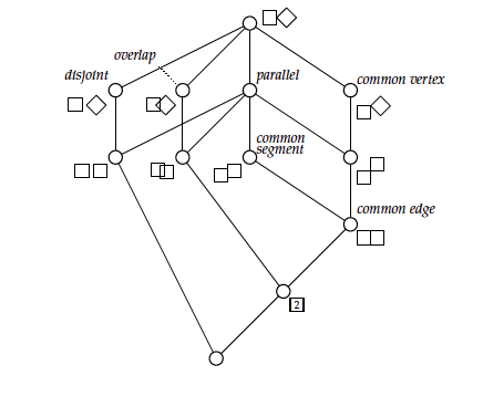
The concept lattice can be plotted using a Hasse diagram and the function plot() inside the ConceptLattice component:
fc_planets$concepts$plot()Warning: You have not installed the 'hasseDiagram' package, which is needed to
plot the lattice.fc_I$concepts$plot()Warning: You have not installed the 'hasseDiagram' package, which is needed to
plot the lattice.If one desires to get the list of concepts printed, or in LaTeX format, just:
# Printing
fc_planets$concepts
A set of 12 concepts:
1: ({Mercury, Venus, Earth, Mars, Jupiter}, {})
2: ({Venus, Earth, Mars, Jupiter}, {moon})
3: ({Earth, Mars, Jupiter}, {far, moon})
4: ({Earth}, {large, far, moon})
5: ({Mars}, {medium, far, moon})
6: ({Mercury, Venus, Jupiter}, {small})
7: ({Venus, Jupiter}, {small, moon})
8: ({Jupiter}, {small, far, moon})
9: ({Mercury, Venus}, {small, near})
10: ({Mercury}, {small, near, no_moon})
11: ({Venus}, {small, near, moon})
12: ({}, {small, medium, large, near, far, moon, no_moon})# LaTeX
fc_planets$concepts$to_latex()Note: You must include the following commands in you LaTeX document:
\usepackage{amsmath}\newcommand{\el}[2]{\ensuremath{^{#2\!\!}/{#1}}}\begin{longtable*}{lll}
1: &$\left(\,\left\{\mathrm{Mercury}, \mathrm{Venus}, \mathrm{Earth}, \mathrm{Mars}, \mathrm{Jupiter}\right\},\right.$&$\left.\ensuremath{\varnothing}\,\right)$\\
2: &$\left(\,\left\{\mathrm{Venus}, \mathrm{Earth}, \mathrm{Mars}, \mathrm{Jupiter}\right\},\right.$&$\left.\left\{\mathrm{moon}\right\}\,\right)$\\
3: &$\left(\,\left\{\mathrm{Earth}, \mathrm{Mars}, \mathrm{Jupiter}\right\},\right.$&$\left.\left\{\mathrm{far}, \mathrm{moon}\right\}\,\right)$\\
4: &$\left(\,\left\{\mathrm{Earth}\right\},\right.$&$\left.\left\{\mathrm{large}, \mathrm{far}, \mathrm{moon}\right\}\,\right)$\\
5: &$\left(\,\left\{\mathrm{Mars}\right\},\right.$&$\left.\left\{\mathrm{medium}, \mathrm{far}, \mathrm{moon}\right\}\,\right)$\\
6: &$\left(\,\left\{\mathrm{Mercury}, \mathrm{Venus}, \mathrm{Jupiter}\right\},\right.$&$\left.\left\{\mathrm{small}\right\}\,\right)$\\
7: &$\left(\,\left\{\mathrm{Venus}, \mathrm{Jupiter}\right\},\right.$&$\left.\left\{\mathrm{small}, \mathrm{moon}\right\}\,\right)$\\
8: &$\left(\,\left\{\mathrm{Jupiter}\right\},\right.$&$\left.\left\{\mathrm{small}, \mathrm{far}, \mathrm{moon}\right\}\,\right)$\\
9: &$\left(\,\left\{\mathrm{Mercury}, \mathrm{Venus}\right\},\right.$&$\left.\left\{\mathrm{small}, \mathrm{near}\right\}\,\right)$\\
10: &$\left(\,\left\{\mathrm{Mercury}\right\},\right.$&$\left.\left\{\mathrm{small}, \mathrm{near}, \mathrm{no\_moon}\right\}\,\right)$\\
11: &$\left(\,\left\{\mathrm{Venus}\right\},\right.$&$\left.\left\{\mathrm{small}, \mathrm{near}, \mathrm{moon}\right\}\,\right)$\\
12: &$\left(\,\ensuremath{\varnothing},\right.$&$\left.\left\{\mathrm{small}, \mathrm{medium}, \mathrm{large}, \mathrm{near}, \mathrm{far}, \mathrm{moon}, \mathrm{no\_moon}\right\}\,\right)$\\
\end{longtable*}For a ConceptLattice, one may want to retrieve particular concepts, using a subsetting as in R:
fc_planets$concepts[2:3]A set of 2 concepts:
1: ({Venus, Earth, Mars, Jupiter}, {moon})
2: ({Earth, Mars, Jupiter}, {far, moon})Or get all the extents and all the intents of all concepts, as sparse matrices:
fc_planets$concepts$extents()5 x 12 sparse Matrix of class "dgCMatrix"
[1,] 1 . . . . 1 . . 1 1 . .
[2,] 1 1 . . . 1 1 . 1 . 1 .
[3,] 1 1 1 1 . . . . . . . .
[4,] 1 1 1 . 1 . . . . . . .
[5,] 1 1 1 . . 1 1 1 . . . .fc_planets$concepts$intents()7 x 12 sparse Matrix of class "dgCMatrix"
[1,] . . . . . 1 1 1 1 1 1 1
[2,] . . . . 1 . . . . . . 1
[3,] . . . 1 . . . . . . . 1
[4,] . . . . . . . . 1 1 1 1
[5,] . . 1 1 1 . . 1 . . . 1
[6,] . 1 1 1 1 . 1 1 . . 1 1
[7,] . . . . . . . . . 1 . 1First, the support of an itemset is:
\[ supp(X)=\frac{X^\prime}{G} \]
The support of a concept $\langle A, B\rangle$ (A is the extent of the concept and B is the intent) is the cardinality (relative) of the extent - number of objects of the extent.
The support of concepts can be computed using the function support():
fc_planets$concepts$support() [1] 1.0000000 0.7777778 0.5555556 0.2222222 0.2222222 0.5555556 0.3333333
[8] 0.1111111 0.4444444 0.2222222 0.2222222 0.0000000The support of itemsets and concepts is used to mine all the knowledge: Algorithm Titanic (computing iceberg concept lattices)
When the concept lattice is too large, it can be useful in certain occasions to just work with a sublattice of the complete lattice. To this end, we use the sublattice() function.
For instance, to build the sublattice of those concepts with support greater than 0.5, we can do:
# Get the index of those concepts with support
# greater than the threshold
idx <- which(fc_I$concepts$support() > 0.2)
# Build the sublattice
sublattice <- fc_I$concepts$sublattice(idx)
sublattice
A set of 13 concepts:
1: ({O1, O2, O3, O4, O5}, {})
2: ({O1, O4, O5}, {P4 [0.5]})
3: ({O1, O4}, {P4 [0.5], P5 [0.5]})
4: ({O1, O2, O5}, {P3 [0.5]})
5: ({O1, O5}, {P3 [0.5], P4 [0.5]})
6: ({O1}, {P3 [0.5], P4 [0.5], P5})
7: ({O1 [0.5], O2, O5}, {P3})
8: ({O1 [0.5], O5}, {P3, P4 [0.5]})
9: ({O1 [0.5]}, {P3, P4, P5})
10: ({O2, O3}, {P1 [0.5], P2 [0.5]})
11: ({O3}, {P1 [0.5], P2 [0.5], P6})
12: ({O2}, {P1, P2, P3})
13: ({}, {P1, P2, P3, P4, P5, P6})And we can plot just the sublattice:
sublattice$plot()Warning: You have not installed the 'hasseDiagram' package, which is needed to
plot the lattice.It may be interesting to use the notions of subconcept and superconcept. Given a concept, we can compute all its subconcepts and all its superconcepts:
# The fifth concept
C <- fc_planets$concepts[5]
C
A set of 1 concepts:
1: ({Mars}, {medium, far, moon})# Its subconcepts:
fc_planets$concepts$subconcepts(C)A set of 2 concepts:
1: ({Mars}, {medium, far, moon})
2: ({}, {small, medium, large, near, far, moon, no_moon})# And its superconcepts:
fc_planets$concepts$superconcepts(C)A set of 4 concepts:
1: ({Mercury, Venus, Earth, Mars, Jupiter}, {})
2: ({Venus, Earth, Mars, Jupiter}, {moon})
3: ({Earth, Mars, Jupiter}, {far, moon})
4: ({Mars}, {medium, far, moon})Also, we can define infimum and supremum of a set of concepts as the greatest common subconcept of all the given concepts, and the lowest common superconcept of them, and can be computed by:
# A list of concepts
C <- fc_planets$concepts[5:7]
C
A set of 3 concepts:
1: ({Mars}, {medium, far, moon})
2: ({Mercury, Venus, Jupiter}, {small})
3: ({Venus, Jupiter}, {small, moon})# Supremum of the concepts in C
fc_planets$concepts$supremum(C)({Mercury, Venus, Earth, Mars, Jupiter}, {})# Infimum of the concepts in C
fc_planets$concepts$infimum(C)({}, {small, medium, large, near, far, moon, no_moon})Theorem:
In a complete lattice, an element is called supremum-irreducible or join-irreducible if it cannot be written as the supremum of other elements and infimum-irreducible or meet-irreducible if it can not be expressed as the infimum of other elements.
The irreducible elements with respect to join (supremum) and meet (infimum) can be computed for a given concept lattice:
fc_planets$concepts$join_irreducibles()A set of 5 concepts:
1: ({Earth}, {large, far, moon})
2: ({Mars}, {medium, far, moon})
3: ({Jupiter}, {small, far, moon})
4: ({Mercury}, {small, near, no_moon})
5: ({Venus}, {small, near, moon})fc_planets$concepts$meet_irreducibles()A set of 7 concepts:
1: ({Venus, Earth, Mars, Jupiter}, {moon})
2: ({Earth, Mars, Jupiter}, {far, moon})
3: ({Earth}, {large, far, moon})
4: ({Mars}, {medium, far, moon})
5: ({Mercury, Venus, Jupiter}, {small})
6: ({Mercury, Venus}, {small, near})
7: ({Mercury}, {small, near, no_moon})This are the concepts used to build the standard context, mentioned above.
10.0.5 Implications
The datasets in this section come from this paper.
The crisp version of the data appears in Table 3 in the mentioned paper.
objects <- paste0("O", 1:6)
n_objects <- length(objects)

attributes <- paste0("P", 1:6)
n_attributes <- length(attributes)

I <- matrix(data = c(0, 1, 1, 0, 0, 1,
                     1, 1, 1, 0, 0, 0,
                     1, 1, 0, 0, 1, 0,
                     1, 0, 0, 1, 1, 0,
                     1, 0, 0, 1, 0, 0,
                     0, 0, 1, 0, 0, 0),
            nrow = n_objects,
            byrow = FALSE)

colnames(I) <- attributes
rownames(I) <- objects
Once we create the formal context object, with the previous data matrix I, we can compute all concepts and implications using Ganter’s algorithm:
fc <- FormalContext$new(I)

# Compute implications
fc$find_implications(verbose = FALSE)

# Cardinality and mean size in the ruleset
fc$implications$cardinality()
[1] 7sizes <- fc$implications$size()
colMeans(sizes) LHS RHS
2.142857 1.857143 The obtained implications are:
fc$implicationsImplication set with 7 implications.
Rule 1: {P6} -> {P1, P2}
Rule 2: {P5} -> {P4}
Rule 3: {P3, P4, P5} -> {P2}
Rule 4: {P2, P4} -> {P3, P5}
Rule 5: {P1, P4} -> {P2, P3, P5, P6}
Rule 6: {P1, P3} -> {P2}
Rule 7: {P1, P2, P3, P6} -> {P4, P5}We provide functions to plot both the concept lattice and the formal context:
# Visualize the concept lattice
fc$concepts$plot()
Warning: You have not installed the 'hasseDiagram' package, which is needed to
plot the lattice.# And the formal context
fc$plot()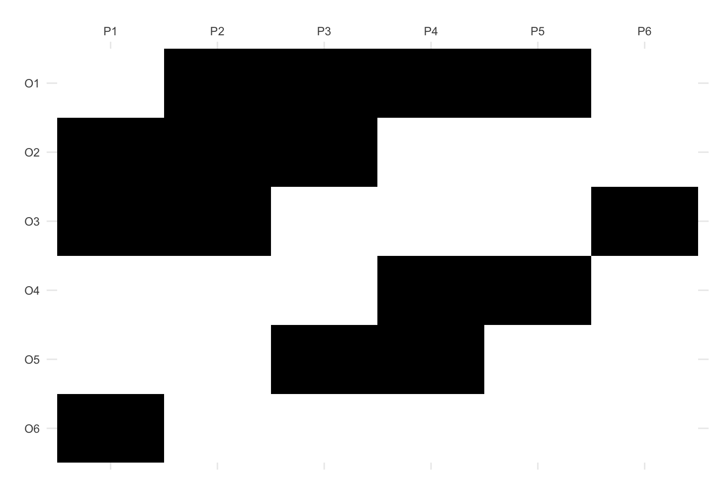
Let us apply some simplification rules to achieve redudancy Removal:
fc$implications$apply_rules(rules = c("composition",
                                      "generalization",
                                      "simplification"),
                            parallelize = FALSE)
Processing batch--> Composition: from 7 to 7.--> Generalization: from 7 to 7.--> Simplification: from 7 to 7.# Compute cardinality and size in the transformed ruleset:
fc$implications$cardinality()[1] 7sizes <- fc$implications$size()
colMeans(sizes) LHS RHS
1.714286 1.857143 The transformed ruleset:
fc$implicationsImplication set with 7 implications.
Rule 1: {P6} -> {P1, P2}
Rule 2: {P5} -> {P4}
Rule 3: {P3, P5} -> {P2}
Rule 4: {P2, P4} -> {P3, P5}
Rule 5: {P1, P4} -> {P2, P3, P5, P6}
Rule 6: {P1, P3} -> {P2}
Rule 7: {P3, P6} -> {P4, P5}The fuzzy version of the data appears in Table 2 in the mentioned paper.
objects <- paste0("O", 1:6)
n_objects <- length(objects)

attributes <- paste0("P", 1:6)
n_attributes <- length(attributes)

I <- matrix(data = c(0, 1, 0.5, 0, 0, 0.5,
                     1, 1, 0.5, 0, 0, 0,
                     0.5, 1, 0, 0, 1, 0,
                     0.5, 0, 0, 1, 0.5, 0,
                     1, 0, 0, 0.5, 0, 0,
                     0, 0, 1, 0, 0, 0),
            nrow = n_objects,
            byrow = FALSE)

colnames(I) <- attributes
rownames(I) <- objects
As before, we build the formal context object and compute all implications:
fc <- FormalContext$new(I)

# Compute
fc$find_implications(verbose = FALSE)

# Some properties of the ruleset
fc$implications$cardinality()
[1] 12sizes <- fc$implications$size()
colMeans(sizes) LHS RHS
1.541667 1.916667 The extracted ruleset is:
fc$implicationsImplication set with 12 implications.
Rule 1: {P6 [0.5]} -> {P1 [0.5], P2 [0.5], P6}
Rule 2: {P5 [0.5]} -> {P4 [0.5]}
Rule 3: {P3 [0.5], P4 [0.5], P5 [0.5]} -> {P2, P5}
Rule 4: {P3 [0.5], P4} -> {P3}
Rule 5: {P2 [0.5], P4 [0.5]} -> {P2, P3 [0.5], P5}
Rule 6: {P2 [0.5], P3 [0.5]} -> {P2}
Rule 7: {P2, P3, P4 [0.5], P5} -> {P4}
Rule 8: {P1 [0.5], P4 [0.5]} -> {P1, P2, P3, P4, P5, P6}
Rule 9: {P1 [0.5], P3 [0.5]} -> {P1, P2, P3}
Rule 10: {P1 [0.5], P2} -> {P1}
Rule 11: {P1, P2 [0.5]} -> {P2}
Rule 12: {P1, P2, P3, P6} -> {P4, P5}Let us plot the concept lattice and the formal context.
# Visualize the concept lattice
fc$concepts$plot()
Warning: You have not installed the 'hasseDiagram' package, which is needed to
plot the lattice.# And the formal context
fc$plot()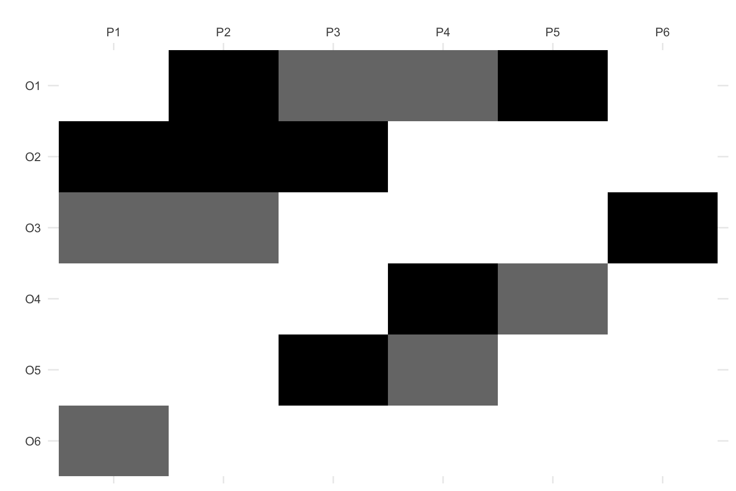
Let us apply some functions to remove redudancies in the set of implications:
fc$implications$apply_rules(rules = c("composition"),
                            reorder = FALSE,
                            parallelize = FALSE)
Processing batch--> Composition: from 12 to 12.fc$implications$cardinality()[1] 12sizes <- fc$implications$size()
colMeans(sizes) LHS RHS
1.541667 1.916667 fc$implications$apply_rules(rules = c("simplification"),
reorder = FALSE,
parallelize = FALSE)Processing batch--> Simplification: from 12 to 12.fc$implications$cardinality()[1] 12sizes <- fc$implications$size()
colMeans(sizes) LHS RHS
1.458333 1.916667 fc$implications$apply_rules(rules = c("generalization"),
reorder = FALSE,
parallelize = FALSE)Processing batch--> Generalization: from 12 to 12.fc$implications$cardinality()[1] 12sizes <- fc$implications$size()
colMeans(sizes) LHS RHS
1.458333 1.916667 The reduced ruleset is:
fc$implicationsImplication set with 12 implications.
Rule 1: {P6 [0.5]} -> {P1 [0.5], P2 [0.5], P6}
Rule 2: {P5 [0.5]} -> {P4 [0.5]}
Rule 3: {P3 [0.5], P5 [0.5]} -> {P2, P5}
Rule 4: {P3 [0.5], P4} -> {P3}
Rule 5: {P2 [0.5], P4 [0.5]} -> {P2, P3 [0.5], P5}
Rule 6: {P2 [0.5], P3 [0.5]} -> {P2}
Rule 7: {P2, P3, P5} -> {P4}
Rule 8: {P1 [0.5], P4 [0.5]} -> {P1, P2, P3, P4, P5, P6}
Rule 9: {P1 [0.5], P3 [0.5]} -> {P1, P2, P3}
Rule 10: {P1 [0.5], P2} -> {P1}
Rule 11: {P1, P2 [0.5]} -> {P2}
Rule 12: {P1, P2, P3, P6} -> {P4, P5}Let us show how to compute the closure of a set S with respect to the implication set.
S <-  Set$new(attributes = fc$attributes)
S$assign(P2 = 0.5, P3 = 0.5)
S
{P2 [0.5], P3 [0.5]}fc$implications$closure(S)$closure
{P2, P3 [0.5]}